How to solve Multi-Label Classification Problems in Deep Learning with Tensorflow & Keras?

This is the fourth part of the “How to solve Classification Problems in Keras?” series. Before starting this tutorial, I strongly suggest you go over Part A: Classification with Keras to learn all related concepts.

In this tutorial, we will focus on how to solve Multi-Label Classification Problems in Deep Learning with Tensorflow & Keras. First, we will download a sample Multi-label dataset. In multi-label classification problems, we mostly encode the true labels with multi-hot vectors. We will experiment with combinations of various last layer’s activation functions and loss functions of a Keras CNN model and we will observe the effects on the model’s performance.

During experiments, we will discuss the relationship between Activation & Loss functions, label encodings, and accuracy metrics in detail. We will understand why sometimes we could get surprising results when using different parameter settings other than the generally recommended ones. As a result, we will gain insight into activation and loss functions and their interactions. In the end, we will summarize the experiment results in a cheat table.

You can access the code at Colab and all the posts of the classification tutorial series at muratkarakaya.net. You can watch all these parts on YouTube in ENGLISH or TURKISH as well.

If you would like to follow up on Deep Learning tutorials, please subscribe to my YouTube Channel or follow my blog on muratkarakaya.net. Do not forget to turn on Notifications so that you will be notified when new parts are uploaded.

If you are ready, let’s get started!

Photo by Luca Martini on Unsplash

1. Download & Process the Dataset

Download

First, let’s load the data from Image Data for Multi-Instance Multi-Label Learning

The image collection contains 2000 natural scene images.

!wget https://www.dropbox.com/s/0htmeoie69q650p/miml_dataset.zip

Unzip the data

!unzip -o -q miml_dataset.ziptime: 442 ms (started: 2021-01-06 09:30:04 +00:00)

Check the metadata

df=pd.read_csv("./miml_dataset/miml_labels_1.csv")
df.head()

time: 44.9 ms (started: 2021-01-06 09:30:04 +00:00)

Record the labels

LABELS=["desert", "mountains", "sea", "sunset", "trees"]time: 1 ms (started: 2021-01-06 09:30:04 +00:00)

Prepare the Data Pipeline by using tf.data

You can learn how to use tf.data to create your data pipeline using the link given in video descriptions.

Create a file list using glob

data_dir = pathlib.Path("miml_dataset")
filenames = list(data_dir.glob('images/*.jpg'))
fnames=[]
for fname in filenames:
  fnames.append(str(fname))time: 21.8 ms (started: 2021-01-06 09:30:04 +00:00)ds_size= len(fnames)
print("Number of images in folders: ", ds_size)

number_of_selected_samples=2000
filelist_ds = tf.data.Dataset.from_tensor_slices(fnames[:number_of_selected_samples])

ds_size= filelist_ds.cardinality().numpy()
print("Number of selected samples for dataset: ", ds_size)Number of images in folders:  2000
Number of selected samples for dataset:  2000
time: 22.6 ms (started: 2021-01-06 09:30:04 +00:00)def get_label(file_path):
  parts = tf.strings.split(file_path, '/')
  file_name= parts[-1]
  labels= df[df["Filenames"]==file_name][LABELS].to_numpy().squeeze()
  return tf.convert_to_tensor(labels)time: 2.87 ms (started: 2021-01-06 09:30:04 +00:00)

Let’s resize and scale the images so that we can save time in training

IMG_WIDTH, IMG_HEIGHT = 64 , 64
def decode_img(img):
  #color images
  img = tf.image.decode_jpeg(img, channels=3) 
  #convert unit8 tensor to floats in the [0,1]range
  img = tf.image.convert_image_dtype(img, tf.float32) 
  #resize 
  return tf.image.resize(img, [IMG_WIDTH, IMG_HEIGHT])time: 3.55 ms (started: 2021-01-06 09:30:04 +00:00)

Combine the images with labels

def combine_images_labels(file_path: tf.Tensor):
  label = get_label(file_path)
  img = tf.io.read_file(file_path)
  img = decode_img(img)
  return img, labeltime: 3.76 ms (started: 2021-01-06 09:30:04 +00:00)

Decide the train-test split

train_ratio = 0.80
ds_train=filelist_ds.take(ds_size*train_ratio)
ds_test=filelist_ds.skip(ds_size*train_ratio)time: 6.65 ms (started: 2021-01-06 09:30:04 +00:00)

Decide the batch size

BATCH_SIZE=64time: 760 µs (started: 2021-01-06 09:30:04 +00:00)

Pre-process all the images

ds_train=ds_train.map(lambda x: tf.py_function(func=combine_images_labels,
          inp=[x], Tout=(tf.float32,tf.int64)),
          num_parallel_calls=tf.data.AUTOTUNE,
          deterministic=False)time: 69.9 ms (started: 2021-01-06 09:30:04 +00:00)ds_test= ds_test.map(lambda x: tf.py_function(func=combine_images_labels,
          inp=[x], Tout=(tf.float32,tf.int64)),
          num_parallel_calls=tf.data.AUTOTUNE,
          deterministic=False)time: 11.7 ms (started: 2021-01-06 09:30:04 +00:00)

Convert multi-hot labels to string labels

def covert_onehot_string_labels(label_string,label_onehot):
  labels=[]
  for i, label in  enumerate(label_string):
     if label_onehot[i]:
       labels.append(label)
  if len(labels)==0:
    labels.append("NONE")
  return labelstime: 4.32 ms (started: 2021-01-06 09:30:04 +00:00)

Show some samples from the data pipeline

def show_samples(dataset):
  fig=plt.figure(figsize=(16, 16))
  columns = 3
  rows = 3
  print(columns*rows,"samples from the dataset")
  i=1
  for a,b in dataset.take(columns*rows): 
    fig.add_subplot(rows, columns, i)
    plt.imshow(np.squeeze(a))
    plt.title("image shape:"+ str(a.shape)+" ("+str(b.numpy()) +") "+ 
              str(covert_onehot_string_labels(LABELS,b.numpy())))
    i=i+1
  plt.show()
show_samples(ds_test)9 samples from the dataset

time: 7.8 s (started: 2021-01-06 09:30:04 +00:00)

Notice that above, the True (Actual) Labels are encoded with Multi-hot vectors

Prepare the data pipeline by setting batch size & buffer size using tf.data

#buffer_size = ds_train_resize_scale.cardinality().numpy()/10
#ds_resize_scale_batched=ds_raw.repeat(3).shuffle(buffer_size=buffer_size).batch(64, )

ds_train_batched=ds_train.batch(BATCH_SIZE).cache().prefetch(tf.data.experimental.AUTOTUNE) 
ds_test_batched=ds_test.batch(BATCH_SIZE).cache().prefetch(tf.data.experimental.AUTOTUNE)

print("Number of batches in train: ", ds_train_batched.cardinality().numpy())
print("Number of batches in test: ", ds_test_batched.cardinality().numpy())Number of batches in train:  25
Number of batches in test:  7
time: 10.6 ms (started: 2021-01-06 09:30:12 +00:00)

2. Create a Keras CNN model by using Transfer learning

Import VGG16

To train fast, let’s use Transfer Learning by importing VGG16

base_model = keras.applications.VGG16(
    weights='imagenet',  # Load weights pre-trained on ImageNet.
    input_shape=(64, 64, 3), # VGG16 expects min 32 x 32
    include_top=False)  # Do not include the ImageNet classifier at the top.
base_model.trainable = Falsetime: 328 ms (started: 2021-01-06 10:00:22 +00:00)

Create the classification model

number_of_classes = 5time: 1.17 ms (started: 2021-01-06 10:00:23 +00:00)inputs = keras.Input(shape=(64, 64, 3))
x = base_model(inputs, training=False)
x = keras.layers.GlobalAveragePooling2D()(x)
initializer = tf.keras.initializers.GlorotUniform(seed=42)

activation =  tf.keras.activations.sigmoid #None  # tf.keras.activations.sigmoid or softmax

outputs = keras.layers.Dense(number_of_classes,
                             kernel_initializer=initializer,
                             activation=activation)(x) 
model = keras.Model(inputs, outputs)time: 83.3 ms (started: 2021-01-06 10:00:23 +00:00)

Pay attention:

The last layer has number_of_classes units. So the output (y_pred) will be a vector with number_of_classes dimension.
For the last layer, the activation function can be:
None
sigmoid
softmax
When there is no activation function is used in the model’s last layer, we need to set from_logits=True in cross-entropy loss functions. Thus, cross-entropy loss functions will apply a sigmoid transformation on predicted label values by themselves:

3. Compile & Train

model.compile(optimizer=keras.optimizers.Adam(),
              loss=keras.losses.BinaryCrossentropy(), # default from_logits=False
              metrics=[keras.metrics.BinaryAccuracy()])time: 19.7 ms (started: 2021-01-06 10:00:23 +00:00)

IMPORTANT: We need to use keras.metrics.BinaryAccuracy() for measuring the accuracy since it calculates how often predictions match binary labels.

As we are dealing with multi-label classification and true labels are encoded multi-hot, we need to compare ***pairwise (binary!)***: each element of prediction with the corresponding element of true labels.

Try & See

Now, we can try and see the performance of the model by using a combination of activation and loss functions.

Note: First Epoch (preparing data pipeline) takes 673 seconds on Colab GPU. Next epochs takes only 1 second.

model.fit(ds_train_batched, validation_data=ds_test_batched, epochs=100)Epoch 1/100
25/25 [==============================] - 2s 37ms/step - loss: 0.6444 - binary_accuracy: 0.6206 - val_loss: 0.5407 - val_binary_accuracy: 0.7490
Epoch 2/100
25/25 [==============================] - 1s 22ms/step - loss: 0.5284 - binary_accuracy: 0.7576 - val_loss: 0.5058 - val_binary_accuracy: 0.7625
******
Epoch 99/100
25/25 [==============================] - 1s 23ms/step - loss: 0.2514 - binary_accuracy: 0.8981 - val_loss: 0.2939 - val_binary_accuracy: 0.8715
Epoch 100/100
25/25 [==============================] - 1s 23ms/step - loss: 0.2508 - binary_accuracy: 0.8984 - val_loss: 0.2937 - val_binary_accuracy: 0.8710

4. Evaluate the model

ds= ds_test_batched
print("Test Accuracy: ", model.evaluate(ds)[1])7/7 [==============================] - 0s 15ms/step - loss: 0.2937 - binary_accuracy: 0.8710
Test Accuracy:  0.8710000514984131
time: 131 ms (started: 2021-01-06 10:01:21 +00:00)

10 sample predictions

ds=ds_test
predictions= model.predict(ds.batch(batch_size=10).take(1))
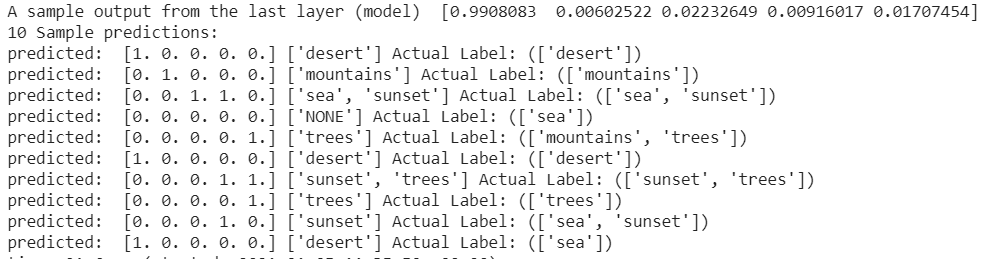
print("A sample output from the last layer (model) ", predictions[0])
y=[]
print("10 Sample predictions:")
for (pred,(a,b)) in zip(predictions,ds.take(10)):
  
  pred[pred>0.5]=1
  pred[pred<=0.5]=0
  print("predicted: " ,pred, str(covert_onehot_string_labels(LABELS, pred)),  
        "Actual Label: ("+str(covert_onehot_string_labels(LABELS,b.numpy())) +")")
  y.append(b.numpy())
A sample output from the last layer (model)  [0.08407215 0.25767672 0.1277057  0.00502216 0.5063773 ]
10 Sample predictions:
predicted:  [0. 0. 0. 0. 1.] ['trees'] Actual Label: (['desert'])
predicted:  [0. 0. 0. 1. 0.] ['sunset'] Actual Label: (['sunset'])
predicted:  [0. 0. 0. 0. 1.] ['trees'] Actual Label: (['trees'])
predicted:  [0. 0. 0. 1. 0.] ['sunset'] Actual Label: (['sea', 'sunset', 'trees'])
predicted:  [0. 0. 0. 0. 1.] ['trees'] Actual Label: (['trees'])
predicted:  [0. 0. 0. 0. 1.] ['trees'] Actual Label: (['mountains'])
predicted:  [0. 0. 0. 0. 1.] ['trees'] Actual Label: (['trees'])
predicted:  [0. 0. 1. 1. 0.] ['sea', 'sunset'] Actual Label: (['sea', 'sunset'])
predicted:  [0. 0. 0. 1. 0.] ['sunset'] Actual Label: (['desert'])
predicted:  [0. 1. 0. 0. 0.] ['mountains'] Actual Label: (['mountains'])

5. Obtained Results*:

When you run this notebook, most probably you would not get the exact numbers rather you would observe very similar values due to the stochastic nature of ANNs.

6. Observations & Discussions

Why does SparseCategoricalCrossentropy loss functions generate errors?

Because, to encode the true labels, we are using multi-hot vectors.

However, SparseCategoricalCrossentropy expects true labels as an integer number.

Moreover, we can NOT encode multi-labels as an integer since there would be more than one label for a sample.

Therefore, the SparseCategoricalCrossentropy loss functions can NOT handle a multi-hot vector!

Why does Sigmoid produce the best performance when BinaryCrossentropy Loss Function is used?

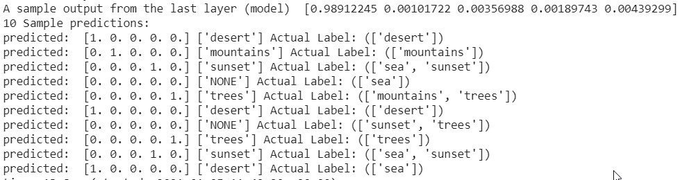
When softmax is applied as the last layer’s activation function, is able to only select a single label as the prediction as softmax normalizes all predicted values as a probability distribution. Only one label could get a higher value than 0.5.
Thus, softmax can only predict a SINGLE class at most! in a multi-label problem! So softmax will miss other true labels which leads to inferior performance compared to sigmoid.

When sigmoid is applied as the last layer’s activation function, it is able to select multiple labels as the prediction as sigmoid normalize each predicted logit values between 0 and 1 independently.

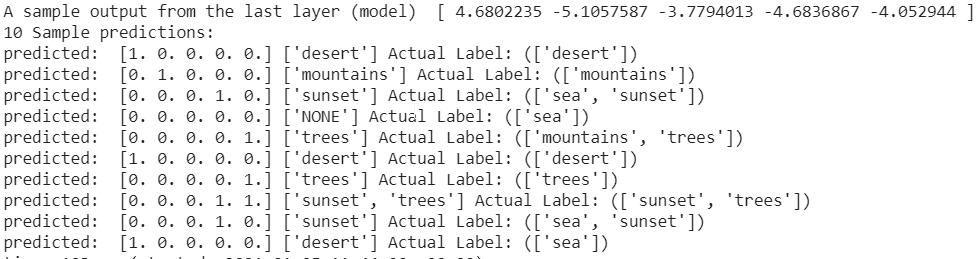
When no activation function (None) is used, each label prediction gets arbitrary numbers from negative infinitive to positive infinitive. BinaryCrossentropy with from_logits parameter is set True automatically applies sigmoid on these logits. Thus, in this case, we have a similar performance compared to the case where we use sigmoid for the last layer's activation function.

Does CategoricalCrossentropy loss function generate good results?

NO! At the above table, it looks like that CategoricalCrossentropy with softmax & sigmoid activation functions generates good results. However, if we observe the predictions closely:

When softmax is applied as the last layer’s activation function, we can only select a single label as the prediction as softmax normalize all predicted values as a probability distribution. Only one label could get higer value than 0.5

Important: Please note that we are using BinaryAccuracy to calculate the accuracy. That is we are comparing true and predicted label vectors by matching one pair at a time! Thus, the prediction vectors with all 0 or all 1 values can lead to considerable good accuracy.

As we see below, after sigmoid transformation the prediction vector has values equal to almost zeros. However, the binary accuracy is 60% since 3 zeros in the true label have been correctly identified!:

# Assume last layer output is as:
y_pred_logit = tf.constant([[-20, -10.0, -44.5, -12.5, -74]], dtype = tf.float32)
print("y_pred_logit:\n", y_pred_logit.numpy())

# and last layer activation function is sigmoid:
y_pred_sigmoid = tf.keras.activations.sigmoid(y_pred_logit)

y_true=[[1, 0, 0, 0, 1]]
y_pred = y_pred_sigmoid
print("\ny_true {} \n\ny_pred by sigmoid {}\n".format(y_true, y_pred))
print("binary_accuracy: ", tf.keras.metrics.binary_accuracy
      (y_true, y_pred).numpy())y_pred_logit:
 [[-20.  -10.  -44.5 -12.5 -74. ]]

y_true [[1, 0, 0, 0, 1]] 

y_pred by sigmoid [[2.0611535e-09 4.5397868e-05 4.7194955e-20 3.7266393e-06 7.2812905e-33]]

binary_accuracy:  [0.6]

When sigmoid is the activation function & loss is computed by CategoricalCrossentropy function, we can NOT select any labels as the prediction because all the predicted values get very close to zero.

When None of the activation functions is selected & loss is computed by CategoricalCrossentropy function, each label prediction gets arbitrary numbers from negative infinitive to positive infinitive. All predicted label values get higher than 0.5. Thus, all labels are selected.