
How to Evaluate a Classifier Trained with an Imbalanced Dataset? Why Accuracy is not Enough?
Author: Murat Karakaya
Date created: 19 May 2020
Last modified: 09 Dec 2021
Description: In this tutorial series, we will discuss how to evaluate a classifier trained with an imbalanced dataset. We will see that accuracy metric is not enough to measure the performance of classifiers, especially, when you have an imbalanced dataset. Furthermore, we will implement 8 different classifier models and evaluate their success by comparing the various classification metric results. We will implement the solutions by Python and SciKit Learn library.
Accessible on:
- Murat Karakaya Akademi YouTube Channel in English or Turkish
- muratkarakaya.net
- Google Colab
- Kaggle
- Github
- Github pages
- Github Repo
Parts
I will deliver the content in 3 parts:
- Part A: Fundamentals, Metrics, Synthetic Dataset
- Part B: Dummy Classifiers, Accuracy, Precision, Recall, F1
- Part C: ROC, AUC, Worthless Test, Setting up threshold

Part A: Fundamentals, Metrics, Synthetic Dataset
The Scope:
At the end of the tutorial, we will learn the answers to these questions:
- what is an imbalanced dataset
- what is a dummy classifier
- how to measure the performance of a binary classifier
- how to compare the performances of classification algorithms
- which metrics are meaningful which is useless
- how to interpret the metric scores or graphics
- why “accuracy” is not a good metric
- why a fixed threshold value is not useful
- why 99% accuracy is not enough
- why accuracy is not a good performance metric in some classification tasks
- what about recall, precision & f1
- how to interpret ROC curve & AUC
- which classifier is better among the alternatives
- how to create a random binary classification dataset by SciKit Learn
Furthermore, we will cover the following classification metrics and the related concepts in detail:
- Accuracy
- Recall
- Precision
- F1
- ROC
- ROC AUC
- predict
- predict_proba
- threshold
Definitions
- Synthetic data is information that’s artificially manufactured rather than generated by real-world events. Synthetic data is created algorithmically, and it is used as a stand-in for test datasets of production or operational data, to validate mathematical models and, increasingly, to train machine learning models.
- Imbalanced datasets are a special case for classification problems where the class distribution is not uniform among the classes. That is, a classification data set with skewed class proportions is called imbalanced. Classes that make up a large proportion of the data set are called majority classes. Those that make up a smaller proportion are minority classes.
- Performance metrics, for classification problems, involve comparing the expected class label to the predicted class label or interpreting the predicted probabilities for the class labels for the problem.
- Classification accuracy is the number of correct predictions divided by the total number of predictions.
- Recall is the number of correct positive class predictions divided by the total number of positive samples in the dataset.
- Precision is the number of positive class predictions divided by the number of samples actually belong to the positive class.
- F-Measure (score) is a single score that balances both the precision and recall in one number.
- Sensitivity or True Positive Rate (TPR), also known as recall, is the number of correct positive class predictions divided by the total number of positive samples. (probability of detection)
- False Positive Rate (FPR) is the number of samples incorrectly predicted as positive divided by the total number of positive samples. (probability of false alarm)
- A receiver operating characteristic (ROC) curve is a graphical plot that illustrates the diagnostic ability of a binary classifier system as its discrimination threshold is varied. The ROC curve is created by plotting the true positive rate (TPR) against the false positive rate (FPR) at various threshold settings.
- The Area Under the Curve (AUC) is the measure of the ability of a classifier to distinguish between classes and is used as a summary of the ROC curve.
Sample Problem and Dataset: Predict the Covid-19 test result
Assume that:
- You have collected test data and test results for COVID-19 world-wide
- You know 20 features about all tested subject
- Test result “0: Negative” means that person is healthy
- Test result “1: Positive” means that person is unfortunately sick (COVID-19)
- Our aim is to train a classifier that can most accurately predict the test results using 20 features.
But, first, let’s examine the results from the below figure:
How many tests to find one COVID-19 case?
- What you can notice is that detecting/observing a corona case (positive) per test has a very low probability changing from 0.005 to 0.14.
- The top 5 country average is (5/607) 0.008!
That is, we can continue the above assumptions by adding these ones:
- you collected COVID-19 testing results into a data set,
- in that data set, 99.2% of the test results would be “0: Negative” and 0.8% would be “1: Positive”.
Using these assumptions, below, we will generate a synthetic dataset following the positive/negative test distribution.
After then, we will train 8 different models and compare their performance with various metrics.
In the end,
- we will understand why the accuracy metric is not suitable for classification tasks with imbalanced datasets.
- we will recognize the importance of other metrics such as F1, ROC, AUC, etc.
Import dependencies
import warnings
warnings.filterwarnings('ignore')
from sklearn.datasets import make_classification
from sklearn.dummy import DummyClassifier
from sklearn.linear_model import LogisticRegression
from sklearn.neighbors import KNeighborsClassifier
from sklearn.model_selection import train_test_split
from sklearn.metrics import roc_auc_score
from sklearn.metrics import roc_curve
from sklearn.metrics import classification_report
from matplotlib import pyplot as plt
from sklearn.metrics import accuracy_score
import numpy as np
import pandas as pd
Function to create a synthetic binary classification dataset with specific class distributions
- We will use Scikit Learn make_classification() function with weights parameter which is the proportions of samples assigned to each class.
def makeDataset(size= 1000, negativeClassDistribution=0.5):
  print("Created a random binary dataset with class disributions:")
  # generate 2 class dataset
  X, y = make_classification(n_samples=size, n_classes=2,
                             weights=[negativeClassDistribution],
                             random_state=42)
  print( "class 0 (negative class):{:.2f}% vs class 1 (positive class):{:.2f}% "
                        .format(len(y[y==0])/size*100, len(y[y==1])/size*100))
  print("X shape: ", X.shape, "y shape: ",y.shape)
  print("Five Sample input (X) and output values (y):")
  print("X: ")
  print(pd.DataFrame(X).head())
  print("y: ")
  print(pd.DataFrame(y).head())

  # split into train/test sets
  return train_test_split(X, y, test_size=0.5, random_state=2, stratify=y)
Let’s create a synthetic dataset for a given negative class distribution:
trainX, testX, trainy, testy = makeDataset(size= 2000, negativeClassDistribution = 0.992)
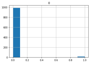
print("y histogram: ")
print(pd.DataFrame(testy).hist())Created a random binary dataset with class disributions:
class 0 (negative class):98.85% vs class 1 (positive class):1.15%
X shape: (2000, 20) y shape: (2000,)
Five Sample input (X) and output values (y):
X:
0 1 2 ... 17 18 19
0 0.231462 1.463082 1.162261 ... -1.663666 -1.407211 3.942331
1 0.522972 0.591132 -0.958704 ... 1.476500 1.873576 1.820967
2 -0.131981 2.935407 -1.633437 ... 2.865920 0.927649 0.983906
3 0.631804 0.043830 1.203177 ... 0.702331 0.467378 -0.047347
4 1.475454 -0.572854 -1.159536 ... -0.464967 0.809846 -0.280024
[5 rows x 20 columns]
y:
0
0 0
1 0
2 0
3 0
4 0
y histogram:
[[<matplotlib.axes._subplots.AxesSubplot object at 0x7f3435edcbd0>]]
Part B: Dummy Classifiers, Accuracy, Precision, Recall, F1
Function to create Dummy Classifiers
- We will use the SciKit Learn DummyClassifier method which is a classifier that makes predictions using simple rules.
- This classifier is useful as a simple baseline to compare with other (real) classifiers.
- Do not use it for real problems.
Function Prototype
class sklearn.dummy.DummyClassifier( strategy=’warn’, random_state=None, constant=None)
Parameters: strategy
default=“stratified”. Strategy to use to generate predictions.
- “stratified”: generates predictions by respecting the training set’s class distribution.
- “most_frequent”: always predicts the most frequent label in the training set.
- “prior”: always predicts the class that maximizes the class prior (like “most_frequent”) and predict_proba returns the class prior.
- “uniform”: generates predictions uniformly at random.
- “constant”: always predicts a constant label that is provided by the user. This is useful for metrics that evaluate a non-majority class
def Dummy(strategy, ax=None, constant=0, showReport=False):
  # no skill model, stratified random class predictions
  model = DummyClassifier(strategy=strategy, constant=constant)
  model.fit(trainX, trainy)
  yhat = model.predict_proba(testX)
  label='DummyClassifier ('+str(strategy)+')'
  if (strategy=='constant'):
    label=label+' '+str(constant)
  print(label)
  if showReport:
    print(classification_report(testy, model.predict(testX)))
  else:
    print("accuracy_score {:.2f}%".format(100*accuracy_score(testy, model.predict(testX))))

  if ax is not None:
    # retrieve just the probabilities for the positive class
    pos_probs = yhat[:, 1]
    # calculate roc auc
    roc_auc = roc_auc_score(testy, pos_probs)
    #print("testy, pos_probs: ", testy, pos_probs)

    # calculate roc curve for model
    fpr, tpr,threshold = roc_curve(testy, pos_probs)
    #print(" fpr, tpr, threshold", fpr, tpr, threshold)
    # plot model roc curve

    ax.set_title('{} ROC AUC {:.3f}'.format(label, roc_auc))
    ax.plot(fpr, tpr, marker='.', label=label)
    # axis labels
    ax.set_xlabel('False Positive Rate')
    ax.set_ylabel('True Positive Rate')
    # show the legend
    ax.legend()
  return ax
Function to use KNN and Logistic Regression classifiers as skillful classifiers
def SkilFul(model, ax=None,   showReport= False, return_tresholds = False):
  # skilled model
  label=str(model)[:15]
  print("A skilled model: "+ label)
  model = model
  model.fit(trainX, trainy)
  yhat = model.predict_proba(testX)

  if showReport:
    print(classification_report(testy, model.predict(testX)))
  else:
    print("accuracy_score {:.2f}%".format(100*accuracy_score(testy, model.predict(testX))))


  # retrieve just the probabilities for the positive class
  # The binary case expects a shape (n_samples,), and the scores must be the scores of
  # the class with the greater label.
  pos_probs = yhat[:, 1]
  #print("yhat \n", yhat.shape)
  # calculate roc auc
  roc_auc = roc_auc_score(testy, pos_probs)
  #print('Logistic ROC AUC %.3f' % roc_auc)

  # calculate roc curve for model
  fpr, tpr, threshold = roc_curve(testy, pos_probs)
  #print(" fpr, tpr, threshold", fpr, tpr, threshold)
  if ax is not None:

    # plot model roc curve
    ax.plot(fpr, tpr, marker='.', label=label)

    ax.set_title('{} ROC AUC {:.3f}'.format(label, roc_auc))

    # axis labels
    ax.set_xlabel('False Positive Rate')
    ax.set_ylabel('True Positive Rate')
    # show the legend
    ax.legend()
  if return_tresholds:
    return ax,fpr, tpr, threshold
  else:
    return ax
“Accuracy” score for all 8 classifiers
Dummy('stratified')
Dummy('most_frequent')
Dummy('prior')
Dummy('uniform')
Dummy('constant', constant=0)
Dummy('constant', constant=1)
SkilFul(model=LogisticRegression())
SkilFul(model=KNeighborsClassifier())DummyClassifier (stratified)
accuracy_score 97.00%
DummyClassifier (most_frequent)
accuracy_score 98.90%
DummyClassifier (prior)
accuracy_score 98.90%
DummyClassifier (uniform)
accuracy_score 46.70%
DummyClassifier (constant) 0
accuracy_score 98.90%
DummyClassifier (constant) 1
accuracy_score 1.10%
A skilled model: LogisticRegress
accuracy_score 99.00%
A skilled model: KNeighborsClass
accuracy_score 98.90%
Observations
- All the classifiers, except DummyClassifier (uniform) & DummyClassifier (constant) 1, achive very high accuracy scores (>97%)!
- DummyClassifier (uniform) yields an accuracy of 53.10% whereas DummyClassifier (constant) 1 produces only 1.30% accuracy, as expected.
Question:
Do you think if we can use all other classifiers in the prediction of positive samples since they have very high accuracy?
Keep your answer in your mind for a moment, and let’s see more results for various metrics :)
More metrics, More Insight: Precision, Recall, F1
We can observe more metrics by using the SciKit Learn classification_report() method.
Before investigating the results remember that there are only 11 positive cases (1) in the test dataset and our aim is to detect possible patients!
So notice the recall values in the reports to understand how many of the positive cases are predicted correctly by looking at the second line of each report

Dummy('stratified',  showReport= True)
Dummy('most_frequent',  showReport= True)
Dummy('prior',  showReport= True)
Dummy('uniform',  showReport= True)
Dummy('constant',  constant=0, showReport= True)
Dummy('constant',  constant=1, showReport= True)
SkilFul(model=LogisticRegression(), showReport= True)
SkilFul(model=KNeighborsClassifier(), showReport= True)DummyClassifier (stratified)
              precision    recall  f1-score   support

           0       0.99      0.99      0.99       989
           1       0.00      0.00      0.00        11

    accuracy                           0.98      1000
   macro avg       0.49      0.49      0.49      1000
weighted avg       0.98      0.98      0.98      1000

DummyClassifier (most_frequent)
              precision    recall  f1-score   support

           0       0.99      1.00      0.99       989
           1       0.00      0.00      0.00        11

    accuracy                           0.99      1000
   macro avg       0.49      0.50      0.50      1000
weighted avg       0.98      0.99      0.98      1000

DummyClassifier (prior)
              precision    recall  f1-score   support

           0       0.99      1.00      0.99       989
           1       0.00      0.00      0.00        11

    accuracy                           0.99      1000
   macro avg       0.49      0.50      0.50      1000
weighted avg       0.98      0.99      0.98      1000

DummyClassifier (uniform)
              precision    recall  f1-score   support

           0       0.99      0.52      0.68       989
           1       0.01      0.55      0.02        11

    accuracy                           0.52      1000
   macro avg       0.50      0.53      0.35      1000
weighted avg       0.98      0.52      0.67      1000

DummyClassifier (constant) 0
              precision    recall  f1-score   support

           0       0.99      1.00      0.99       989
           1       0.00      0.00      0.00        11

    accuracy                           0.99      1000
   macro avg       0.49      0.50      0.50      1000
weighted avg       0.98      0.99      0.98      1000

DummyClassifier (constant) 1
              precision    recall  f1-score   support

           0       0.00      0.00      0.00       989
           1       0.01      1.00      0.02        11

    accuracy                           0.01      1000
   macro avg       0.01      0.50      0.01      1000
weighted avg       0.00      0.01      0.00      1000

A skilled model: LogisticRegress
              precision    recall  f1-score   support

           0       0.99      1.00      0.99       989
           1       1.00      0.09      0.17        11

    accuracy                           0.99      1000
   macro avg       0.99      0.55      0.58      1000
weighted avg       0.99      0.99      0.99      1000

A skilled model: KNeighborsClass
              precision    recall  f1-score   support

           0       0.99      1.00      0.99       989
           1       0.00      0.00      0.00        11

    accuracy                           0.99      1000
   macro avg       0.49      0.50      0.50      1000
weighted avg       0.98      0.99      0.98      1000
Observations
- All the classifiers except DummyClassifier (uniform) & DummyClassifier (constant) 1 are not able to recall (detect) any positive cases at all!
- DummyClassifier (constant) 1 recalls all the positive cases, as expected. Since DummyClassifier (constant) 1 always predicts 1! Thus, according to DummyClassifier (constant) 1, every tested person is positive :)
- DummyClassifier (uniform) recalls the 0.08% of the positive cases. That is DummyClassifier (uniform) correctly classify only 1 positive case (0.08 * 13 = 1.04) out of 13!
Repeated Question:
Do you think if we can use any of these classifiers in the prediction of positive samples since they have very high accuracy?
New Question:
Do you think if we can use any of these classifiers in the prediction of positive samples since they have a very high average F1 score?
Harder Question:
Do you think which classifier is better for our goal with respect to which metric?
Again, keep your answer in your mind for a moment, and let’s see more results for various metrics :)
Part C: ROC, AUC, Worthless Test, Setting up threshold
Receiver Operator Curve (ROC) & Area Under Curve (AUC)
Important Reminders
So far, for any classifier, the threshold value is fixed at 0.5 for deciding a class label
- That is, the class label is decided as “0” if the class probability is less than 0.5
- The class label is decided as “1” if the class probability is greater than or equal to 0.5
In ROC metric we try all possible threshold values for class probabilities to decide class labels
- In ROC, for each possible threshold value, we calculate the True Positive Rate (TPR) and False Positive Rate (FPR) values and draw their values on a plot: the ROC plot
- In the ROC plot, these TPR & FPR pairs generate a curve and we can calculate the Area Under Curve (AUC).
- The AUC score gives an average performance of the classifier when all possible threshold values are considered
Let’s see:
fig, axes = plt.subplots(nrows=2, ncols=4, figsize=(20, 15))
Dummy('stratified', axes[0][0])
Dummy('most_frequent', axes[0][1])
Dummy('prior', axes[0][2])
Dummy('uniform', axes[0][3])
Dummy('constant', axes[1][0], constant=0)
Dummy('constant', axes[1][1], constant=1)
SkilFul(model=LogisticRegression(),ax=axes[1][2])
SkilFul(model=KNeighborsClassifier(),ax=axes[1][3])

plt.show()DummyClassifier (stratified)
accuracy_score 97.80%
DummyClassifier (most_frequent)
accuracy_score 98.90%
DummyClassifier (prior)
accuracy_score 98.90%
DummyClassifier (uniform)
accuracy_score 50.70%
DummyClassifier (constant) 0
accuracy_score 98.90%
DummyClassifier (constant) 1
accuracy_score 1.10%
A skilled model: LogisticRegress
accuracy_score 99.00%
A skilled model: KNeighborsClass
accuracy_score 98.90%
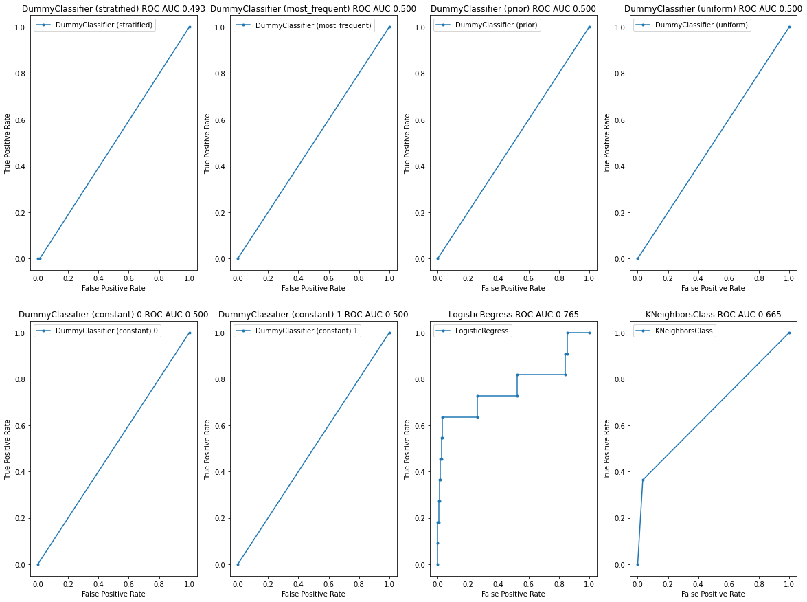
NOTE: THE WORTHLESS TEST
- When we have a complete overlap between the results from the positive and the results from the negative population, we have a worthless test.
- A worthless test has a discriminating ability equal to flipping a coin.
- The ROC curve of the worthless test falls on the diagonal line. It includes the point with 50 % sensitivity and 50 % specificity. The area under the ROC curve (ROC AUC) of the worthless test is 0.5.
Categorization of ROC curves
- As a rule of thumb, the categorizations in TABLE can be used to describe a ROC curve.
Observations
- All the classifiers except LogisticRegress & KNeighborsClass have 0.5. the area under the ROC curve (ROC AUC) score. That is, they are worthless tests. They are useless!
- LogisticRegress has 0.837 ROC AUC score. According to the above table, it is a good classifier for the given dataset!
- KNeighborsClass has a 0.563 ROC AUC score. According to the above table, it is not a good classifier for the given dataset!
New Question:
Do you think if we can use the LogisticRegress classifier in the prediction of positive samples since it has a high ROC AUC score?
Remember that, according to the previous classification reports, the LogisticRegress classifier has not been able to detect a single positive case!

Important Question:
So, why does the LogisticRegress classifier have a high ROC AUC score?
Answer:
- Remember that the above classification report is produced assuming that if the predicted class probability is less than 0.5 threshold value, the predicted label becomes 0:Negative, else 1:Positive!
- However, in the calculation of the ROC AUC score, we care about all possible threshold values!
- That is, there are some threshold values at which the LogisticRegress classifier can predict positive cases correctly!
Please continue with the following code:
model= LogisticRegression()
  label=str(model)[:15]
  print("A skilled model: "+ label)
  model.fit(trainX, trainy)
  yhat = model.predict_proba(testX)
  pos_probs = yhat[:, 1]
  print(classification_report(testy, model.predict(testX)))
  for threshold in np.linspace(0,1,11):
    print("{} tests considered to be POSITIVE when threshold is {:.1} "
    .format(len(pos_probs[pos_probs>=threshold]),threshold))A skilled model: LogisticRegress
              precision    recall  f1-score   support

           0       0.99      1.00      0.99       989
           1       1.00      0.09      0.17        11

    accuracy                           0.99      1000
   macro avg       0.99      0.55      0.58      1000
weighted avg       0.99      0.99      0.99      1000

1000 tests considered to be POSITIVE when threshold is 0e+00
21 tests considered to be POSITIVE when threshold is 0.1
6 tests considered to be POSITIVE when threshold is 0.2
2 tests considered to be POSITIVE when threshold is 0.3
1 tests considered to be POSITIVE when threshold is 0.4
1 tests considered to be POSITIVE when threshold is 0.5
1 tests considered to be POSITIVE when threshold is 0.6
1 tests considered to be POSITIVE when threshold is 0.7
1 tests considered to be POSITIVE when threshold is 0.8
0 tests considered to be POSITIVE when threshold is 0.9
0 tests considered to be POSITIVE when threshold is 1e+00
Above, you can see that by changing threshold values from 0.1 to 1.0, you can end up with different prediction results for positive class!
Actually, you can use the ROC curve information to locate a specific threshold value which provides you with a better recall value for the positive class.
Below, we will observe the TPR and FPR values for the calculated thresholds:
# calculate roc auc
roc_auc = roc_auc_score(testy, pos_probs)
#print('Logistic ROC AUC %.3f' % roc_auc)

# calculate roc curve for model
fpr, tpr, threshold = roc_curve(testy, pos_probs)
print("threshold:","\ttpr: ", "\tfpr")
for current_threshold,current_tpr, current_fpr in zip(threshold,tpr,fpr):
  print("%.3f" %current_threshold,  "\t\t%.3f" %current_tpr,  "\t%.3f"%current_fpr)threshold: 	tpr:  	fpr
1.860 		0.000 	0.000
0.860 		0.091 	0.000
0.311 		0.182 	0.000
0.162 		0.182 	0.009
0.160 		0.273 	0.009
0.138 		0.273 	0.012
0.119 		0.364 	0.012
0.098 		0.364 	0.018
0.092 		0.455 	0.018
0.070 		0.455 	0.027
0.067 		0.545 	0.027
0.061 		0.545 	0.030
0.055 		0.636 	0.030
0.008 		0.636 	0.263
0.007 		0.727 	0.263
0.002 		0.727 	0.525
0.002 		0.818 	0.525
0.000 		0.818 	0.842
0.000 		0.909 	0.842
0.000 		0.909 	0.854
0.000 		1.000 	0.854
0.000 		1.000 	1.000
As you notice from the results above,
- For different threshold values, the model predictions end up with different TPR and FPR.
- While decreasing the threshold values, TPR and FPR increase.
- That is, with lower values of threshold, with even a low probability, we decide that it is a positive class prediction which increases the TPR (recall) and FPR as well.
According to the problem at hand, you can trade off TPR and FPR scores.
Below, we will decrease the threshold down to 0.160 and report the classification metrics:
print("classification report when threshold is default (0.5)")
print(classification_report(testy, model.predict(testX)))
new_threshold=0.160
print("classification report when threshold is changed to ",new_threshold)
y_pred = (model.predict_proba(testX)[:,1] >= new_threshold).astype(bool)
print(classification_report(testy,y_pred))classification report when threshold is default (0.5)
              precision    recall  f1-score   support

           0       0.99      1.00      0.99       989
           1       1.00      0.09      0.17        11

    accuracy                           0.99      1000
   macro avg       0.99      0.55      0.58      1000
weighted avg       0.99      0.99      0.99      1000

classification report when threshold is changed to  0.16
              precision    recall  f1-score   support

           0       0.99      0.99      0.99       989
           1       0.25      0.27      0.26        11

    accuracy                           0.98      1000
   macro avg       0.62      0.63      0.63      1000
weighted avg       0.98      0.98      0.98      1000
According to the above results, when we decrease the threshold:
- For the 1:Positive class, we observe a higher recall (+18%) but a lower precision value (-75%), as expected.
- Accuracy is decreased a little bit: only 1%
- Macro average F1 is increased (5%) whereas Weighted Avgerage F1 is decreased (1%)
You can select different threshold values and observe similar impacts on the results.
If your aim is to increase the positive class’s TPR, you can compromise from the FPR of the positive class.
Conclusions
- Accuracy is NOT always a good metric for classification, esp. if there exists a class imbalanced data set
- Classification report provides details of other metrics: Precision, Recall, and F1 with averaging over classes with respect to several metrics
- However, the Classification report provides results with different metrics for only a fixed threshold value which does not depict the whole performance of a classifier
- The ROC graph is very useful to inspect the ML method skilfulness under all possible threshold values
- The ROC AUC score is important for measuring the performance of a classifier considering various thresholds
- If a classifier has a ROC AUC around 0.5 is useless even with a 99% accuracy!
- Conduct a comprehensive EDA on the data to see if the classes are balanced.
Improve yourself
You can use Precision-Recall Curve to compare the model performances in imbalanced data sets.
If you like this tutorial, please follow the Murat Karakaya Akademi YouTube channel and Medium blog.
Thank you for your patience!
Keep Deep Learning :)
Comments or Questions?
Please share your Comments or Questions.
Thank you in advance.
Do not forget to check out the next parts!
Take care!