
Part E: Text Classification with an Embedding Layer in a Feed-Forward Network
Multi-Topic Text Classification with Various Deep Learning Models
Author: Murat Karakaya
Date created….. 17 09 2021
Date published… 16 03 2022
Last modified…. 16 03 2022
Description: This is the Part E of the tutorial series “Multi-Topic Text Classification with Various Deep Learning Models” which covers all the phases of multi-class text classification:
- Exploratory Data Analysis (EDA),
- Text preprocessing
- TF Data Pipeline
- Keras TextVectorization preprocessing layer
- Multi-class (multi-topic) text classification
- Deep Learning model design & end-to-end model implementation
- Performance evaluation & metrics
- Generating classification report
- Hyper-parameter tuning
- etc.
We will design various Deep Learning models by using
- the Keras Embedding layer,
- Convolutional (Conv1D) layer,
- Recurrent (LSTM) layer,
- Transformer Encoder block, and
- pre-trained transformer (BERT).
We will cover all the topics related to solving Multi-Class Text Classification problems with sample implementations in Python / TensorFlow / Keras environment.
We will use a Kaggle Dataset in which there are 32 topics and more than 400K total reviews.
If you would like to learn more about Deep Learning with practical coding examples,
- Please subscribe to the Murat Karakaya Akademi YouTube Channel or
- Do not forget to turn on notifications so that you will be notified when new parts are uploaded.
- Follow my blog on muratkarakaya.net
You can access all the codes, videos, and posts of this tutorial series from the links below.

PART E: TEXT CLASSIFICATION WITH AN EMBEDDING LAYER IN A FEED-FORWARD NETWORK
In this part, we will use a Keras embedding layer in a Feed-Forward Network (FFN). During training, we will train this embedding layer as well.
As you remember, we have introduced the embedding concept in Part A. You can review the details of embedding and how Deep Learning models apply it for text classification in the following Murat Karakaya Akademi YouTube playlists:
- Word Embedding in Keras
- Word Embedding Hakkında Herşey (in Turkish)
If you are not familiar with the “classification with Deep Learning” topic, you can find the 5-part tutorials in the below Murat Karakaya Akademi YouTube playlists:
- How to solve Classification Problems in Deep Learning with Tensorflow & Keras
- Derin Öğrenmede Sınıflandırma Çeşitleri Nelerdir? Keras ve TensorFlow ile Nasıl Yapılmalı? (in Turkish)
A basic DL model can use an embedding layer as an initial layer and a couple of dense layers for classification, as seen in the below model.

Please remember that in Part D,
- we built a TF data pipeline
- we configured a Keras
TextVectorizationlayer for text preprocessing and tokenization - we adopted the Keras
TextVectorizationlayer onto the training dataset - we applied the Keras
TextVectorizationlayer to the train, validation, and test datasets - we finalized the TF data pipeline by configuring it
In this part, we will use these train, validation, and test datasets.
Keras Embedding Layer
Keras Embedding Layer turns positive integers (indexes) into dense vectors of fixed size.
Important Arguments:
- input_dim: Integer. Size of the vocabulary, i.e. maximum integer index + 1.
- output_dim: Integer. Dimension of the dense embedding.
- input_length: Length of input sequences, when it is constant. This argument is required if you are going to connect Flatten then Dense layers upstream (without it, the shape of the dense outputs cannot be computed).
Input shape: 2D tensor with shape: (batch_size, input_length).
Output shape: 3D tensor with shape: (batch_size, input_length, output_dim).
For more information, visit the Keras official website.
Let’s build a simple model with an embedding layer
I will use the Keras Functional API to build the model. You can learn the details of this API here.
In Part D, thanks to the Keras TextVectorization layer, we converted the reviews into a max_len fixed-size vector of integers.
Therefore, the input layer of the model would expect a sequence of max_len integers.
Moreover, in Part D, we also decided on the size of the dictionary: vocab_size. We will use this parameter to set up the embedding layer.
# Embedding size for each token
embed_dim = 16
# Hidden layer size in feed forward network
feed_forward_dim = 64
def create_model_FFN():
    inputs_tokens = layers.Input(shape=(max_len,), dtype=tf.int32)
    embedding_layer = layers.Embedding(input_dim=vocab_size,
                                       output_dim=embed_dim,
                                       input_length=max_len)
    x = embedding_layer(inputs_tokens)
    x = layers.Flatten()(x)
    dense_layer = layers.Dense(feed_forward_dim, activation='relu')
    x = dense_layer(x)
    x = layers.Dropout(.5)(x)
    outputs = layers.Dense(number_of_categories)(x)

    model = keras.Model(inputs=inputs_tokens, outputs=outputs, name='model_FFN')
    loss_fn = tf.keras.losses.SparseCategoricalCrossentropy(from_logits=True)
    metric_fn  = tf.keras.metrics.SparseCategoricalAccuracy()
    model.compile(optimizer="adam", loss=loss_fn, metrics=metric_fn)
    return model

model_FFN=create_model_FFN()model_FFN.summary()Model: "model_FFN"
_________________________________________________________________
 Layer (type)                Output Shape              Param #
=================================================================
 input_2 (InputLayer)        [(None, 40)]              0

 embedding (Embedding)       (None, 40, 16)            1600000

 flatten (Flatten)           (None, 640)               0

 dense (Dense)               (None, 64)                41024

 dropout (Dropout)           (None, 64)                0

 dense_1 (Dense)             (None, 32)                2080

=================================================================
Total params: 1,643,104
Trainable params: 1,643,104
Non-trainable params: 0
_________________________________________________________________
tf.keras.utils.plot_model(model_FFN,show_shapes=True)

Train
As you know, in Part D, we have the train, validation, and test datasets ready to input any ML/DL models. Now, we will use the train and validation datasets to train the model.
history=model_FFN.fit(train_ds, validation_data=val_ds ,verbose=2, epochs=7)Epoch 1/7
95/95 - 6s - loss: 3.4562 - sparse_categorical_accuracy: 0.0531 - val_loss: 3.4359 - val_sparse_categorical_accuracy: 0.1328 - 6s/epoch - 60ms/step
Epoch 2/7
95/95 - 1s - loss: 3.2865 - sparse_categorical_accuracy: 0.2319 - val_loss: 3.1461 - val_sparse_categorical_accuracy: 0.2937 - 519ms/epoch - 5ms/step
Epoch 3/7
95/95 - 1s - loss: 2.6160 - sparse_categorical_accuracy: 0.4597 - val_loss: 2.3218 - val_sparse_categorical_accuracy: 0.5766 - 512ms/epoch - 5ms/step
Epoch 4/7
95/95 - 1s - loss: 1.6017 - sparse_categorical_accuracy: 0.6891 - val_loss: 1.5879 - val_sparse_categorical_accuracy: 0.7250 - 503ms/epoch - 5ms/step
Epoch 5/7
95/95 - 1s - loss: 0.9447 - sparse_categorical_accuracy: 0.8222 - val_loss: 1.2255 - val_sparse_categorical_accuracy: 0.7578 - 519ms/epoch - 5ms/step
Epoch 6/7
95/95 - 0s - loss: 0.5667 - sparse_categorical_accuracy: 0.9066 - val_loss: 1.0433 - val_sparse_categorical_accuracy: 0.7812 - 493ms/epoch - 5ms/step
Epoch 7/7
95/95 - 0s - loss: 0.3656 - sparse_categorical_accuracy: 0.9444 - val_loss: 0.9470 - val_sparse_categorical_accuracy: 0.7922 - 498ms/epoch - 5ms/step
time: 9.25 s (started: 2022-03-01 12:16:44 +00:00)
Let’s observe the accuracy and the loss values during the training at each epoch:
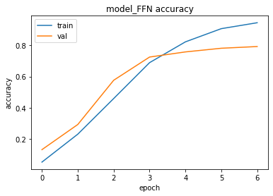

You can observe the underfitting and overfitting behaviors of the model and decide how to handle these situations by tuning the hyper-parameters.
Save the trained model
You can save a Keras model for future use. If you want to learn about saving a Keras model, you can check out my tutorial in English or Turkish.
- TF SavedModel vs HDF5: How to save TF & Keras Models with Custom Objects?
- TF SavedModel vs HDF5: TF & Keras Modellerini Nasıl Saklamalıyız?
tf.keras.models.save_model(model_FFN, 'MultiClassTextClassification_FFN')Test
We can test the trained model with the test dataset:
loss, accuracy = model_FFN.evaluate(test_ds)
print("Test accuracy: ", accuracy)1319/1319 [==============================] - 20s 14ms/step - loss: 0.9454 - sparse_categorical_accuracy: 0.7822
Test accuracy:  0.7822332382202148
time: 19.6 s (started: 2022-03-01 12:16:54 +00:00)
Predictions
We can use the trained model predict() method to predict the class of the given reviews as follows:
preds = model_FFN.predict(test_ds)
preds = preds.argmax(axis=1)time: 2.08 s (started: 2022-03-01 12:17:14 +00:00)
We can also get the actual (true) class of the given reviews as follows:
actuals = test_ds.unbatch().map(lambda x,y: y)
actuals=list(actuals.as_numpy_iterator())time: 21.5 s (started: 2022-03-01 12:17:16 +00:00)
By comparing the preds and the actuals values, we can measure the model performance as below.
Classification Report
Since we are dealing with multi-class text classification, it is a good idea to generate a classification report to observe the performance of the model for each class. We can use the SKLearn classification_report() method to build a text report showing the main classification metrics.
The report is the summary of the precision, recall, and F1 scores for each class.
The reported averages include:
- macro average (averaging the unweighted mean per label),
- weighted average (averaging the support-weighted mean per label),
- sample average (only for multilabel classification),
- micro average (averaging the total true positives, false negatives, and false positives) is only shown for multi-label or multi-class with a subset of classes because it corresponds to accuracy otherwise and would be the same for all metrics.
from sklearn import metrics
print(metrics.classification_report(actuals, preds, digits=4))precision    recall  f1-score   support

           0     0.7651    0.7397    0.7522      2708
           1     0.9261    0.7760    0.8444      2455
           2     0.7431    0.8073    0.7739      2730
           3     0.7478    0.6846    0.7148      2559
           4     0.8234    0.8254    0.8244      2767
           5     0.9853    0.7942    0.8795      2619
           6     0.7741    0.8040    0.7888      2724
           7     0.3566    0.5044    0.4178      2379
           8     0.9659    0.8850    0.9237      2756
           9     0.9601    0.7219    0.8241      2233
          10     0.8999    0.8864    0.8931      2738
          11     0.4577    0.8471    0.5943      2603
          12     0.6731    0.8191    0.7390      2687
          13     0.7845    0.6696    0.7225      2267
          14     0.9442    0.8515    0.8955      2681
          15     0.4817    0.6544    0.5549      2682
          16     0.8431    0.8029    0.8225      2770
          17     0.9079    0.9556    0.9312      2725
          18     0.7222    0.5961    0.6531      2508
          19     0.7111    0.8067    0.7559      2716
          20     0.8709    0.8655    0.8682      2751
          21     0.7579    0.6581    0.7045      2735
          22     0.9314    0.8113    0.8672      2661
          23     0.9468    0.7955    0.8646      2572
          24     0.8791    0.8062    0.8410      2750
          25     0.6670    0.7359    0.6998      2651
          26     0.8484    0.8128    0.8303      2693
          27     0.9519    0.9057    0.9282      2663
          28     0.9488    0.7520    0.8390      2661
          29     0.6972    0.7515    0.7234      2592
          30     0.9252    0.7779    0.8452      2625
          31     0.9441    0.8403    0.8892      2755

    accuracy                         0.7822     84416
   macro avg     0.8076    0.7795    0.7877     84416
weighted avg     0.8088    0.7822    0.7898     84416

time: 670 ms (started: 2022-03-01 12:17:38 +00:00)
In multi-class classification, you need to be careful with the number of samples in each class (support value in the above table). If there is an imbalance among the classes you need to apply some actions.
Moreover, observe the precision, recall, and F1 scores of each class and compare them with the average values of these metrics.
If you would like to learn more about these metrics and how to handle imbalanced datasets, please refer to the following tutorials on the Murat Karakaya Akademi YouTube channel :)
Confusion Matrix
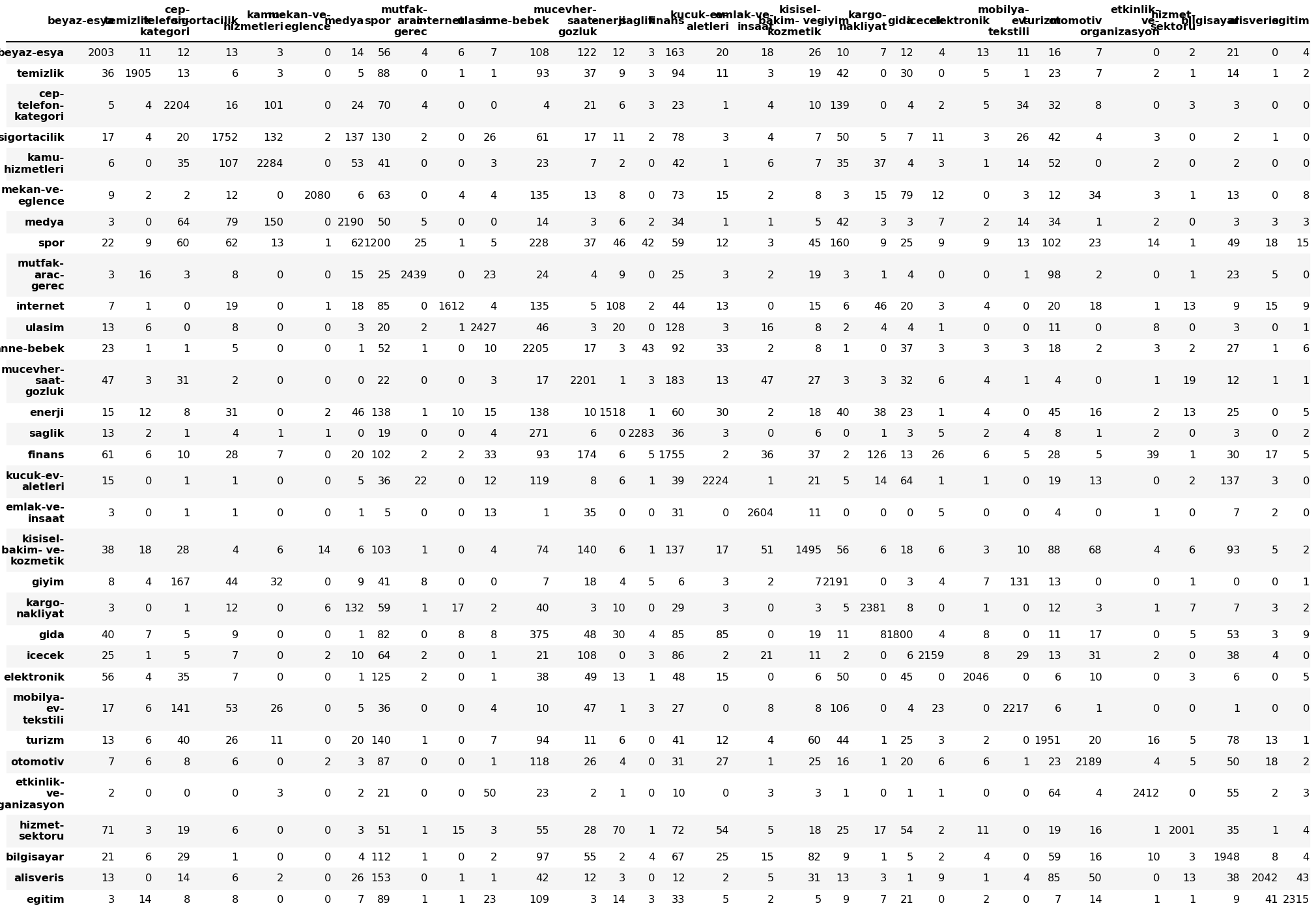
A confusion Matrix is used to know the performance of a Machine learning model at classification. The results are presented in a matrix form. The confusion Matrix gives a comparison between Actual and Predicted values. The numbers on the diagonal are the number of the correct predictions.
Below, you can observe the distribution of predictions over the classes.
We can also visualize the confusion matrix as the ratios of the predictions over the classes. The ratios on the diagonal are the ratios of the correct predictions.
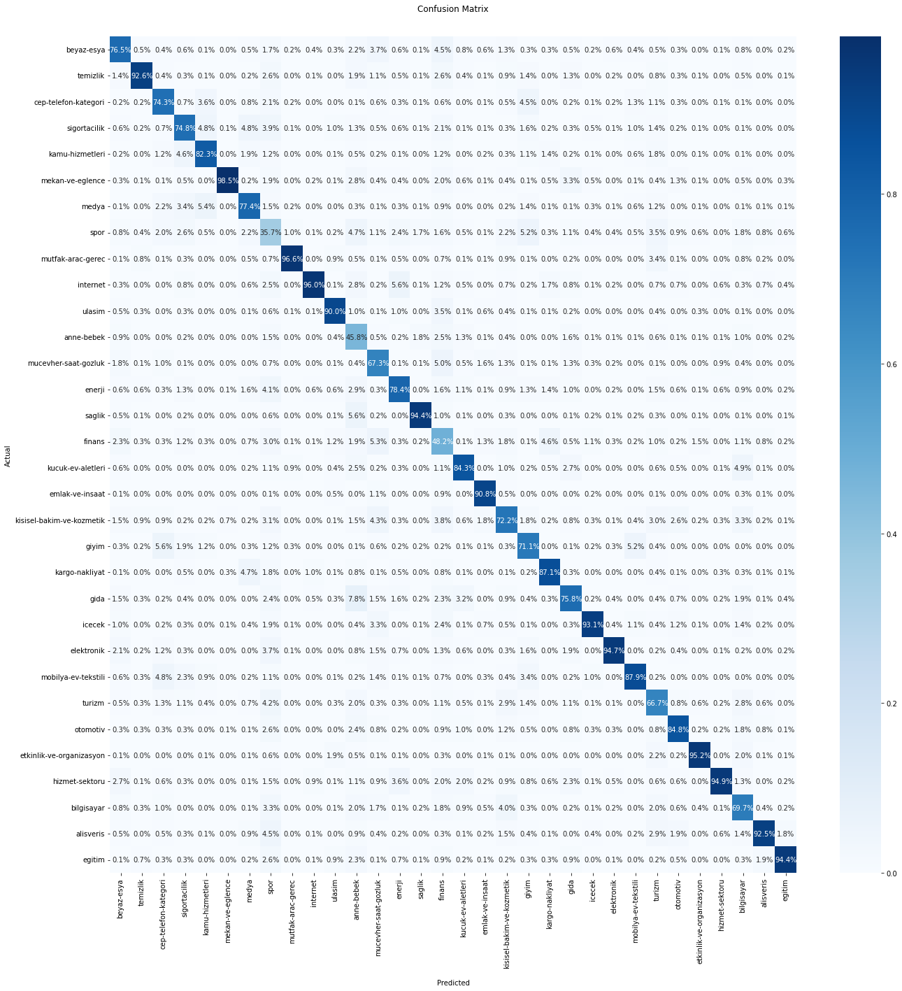
Please, observe the correctly classified sample ratios of each class.
You may need to take some actions for some classes if the correctly predicted sample ratios are relatively low.
Summary
In this part,
- we created a Deep Learning model with an Embedding layer to classify text into multi-classes,
- we trained and tested the model,
- we observed the model performance using Classification Report and Confusion Matrix,
- and we pointed out the importance of the balanced dataset and the performance on each class.
In the next part, we will design another Deep Learning model by using a convolutional layer (Conv1D).
Do you have any questions or comments? Please share them in the comment section.
Thank you for your attention!