Seq2Seq Learning PART F: Encoder-Decoder with Bahdanau & Luong Attention Mechanism

Welcome to Part F of the Seq2Seq Learning Tutorial Series. In this tutorial, we will design an Encoder-Decoder model to handle longer input and output sequences by using two global attention mechanisms: Bahdanau & Luong. During the tutorial, we will be using the Encoder-Decoder model developed in Part C.

First, we will observe that the Basic Encoder-Decoder model will fail to handle long input sequences. Then, we will discuss how to relate each output with all the inputs using the global attention mechanism. We will implement the Bahdanau attention mechanism as a custom layer in Keras by using subclassing. Then, we will integrate the attention layer into the Encoder-Decoder model to efficiently process the longer data. After observing the effect of the attention layer on performance, we will depict the attention between inputs and outputs. Lastly, we will code the Luong attention.

You can access all my SEQ2SEQ Learning videos on Murat Karakaya Akademi Youtube channel in ENGLISH or in TURKISH. You can access all the tutorials in this series from my blog at www.muratkarakaya.net. You can access the whole code on Colab.

If you would like to follow up on Deep Learning tutorials, please subscribe to my YouTube Channel or follow my blog on muratkarakaya.net. Thank you!

If you are ready, let’s get started!

Photo by Bradyn Trollip on Unsplash

REMINDER:

This is the Part F of the Seq2Seq Learning series.
Please check out the previous part to refresh the necessary background knowledge in order to follow this part with ease.

Sample Problem:

In a real-life scenario:

We are given 2 parallel data sets X and y such that X[i] and y[i] have some relationship
For instance: we are given the same book’s text in English (X) and Turkish (y).
Thus the statement X[i] in English is translated into Turkish as y[i] statement
We use the parallel date set to train a seq2seq model which would learn how to convert/transform X[i] to y[i]

Below, we will develop such an encoder-decoder model for fixed-size input and output sequences

The sample problem is to find the reverse of a given sequence

Given sequence X

X=[3, 2, 9, 1]

Output sequence (y) is the reversed input sequence (X)

y=[1, 9, 2, 3]

`Configure the sample problem`

#@title Configure problem

n_timesteps_in =   4
#each input sample has 4 values

n_features = 10   
#each value is one_hot_encoded with 10 0/1

train_size= 2000 
test_size = 200  

For each input sequence (X), selecting  4  random numbers beteen 1 and  10  (0 is reserved )

A sample X 
X=[2, 9, 9, 2]

reversed input sequence (X) is the output sequence (y) 
y=[2, 9, 9, 2]

Each input and output sequences are converted one_hot_encoded format in  10  dimensions
X=[[0 0 1 0 0 0 0 0 0 0]
 [0 0 0 0 0 0 0 0 0 1]
 [0 0 0 0 0 0 0 0 0 1]
 [0 0 1 0 0 0 0 0 0 0]]
y=[[0 0 1 0 0 0 0 0 0 0]
 [0 0 0 0 0 0 0 0 0 1]
 [0 0 0 0 0 0 0 0 0 1]
 [0 0 1 0 0 0 0 0 0 0]]

Generated sequence datasets as follows (batch_size,time_steps, features)
X_train.shape:  (2000, 4, 10) y_train.shape:  (2000, 4, 10)
X_test.shape:  (200, 4, 10) y_test.shape:  (200, 4, 10)
time: 79.7 ms

QUICK LSTM REMINDER

An LSTM layer accepts a series of inputs. Here the input [1, 2, 3, 4] has four-time steps.
The LSTM layer process input step by step:
Time step 1: input 1 is processed and 3 outputs are generated 2 hidden states (the same values) and 1 cell state.
One hidden state is outputted and can be used for prediction or to connect another layer of LSTM
The other hidden state and the cell state are used for the next time step.
At the end of the time steps (here 4), the LSTM layer outputs:
Each time step’s hidden states
Last time step’s hidden state
Last time step’s cell state

You can think above figure as a simple Encoder:

The encoder processes the input and provides the context vector (The last time step’s hidden state + the Last time step’s cell state) for the decoder. *Let’s see the details below.

A BASIC LSTM-BASED ENCODER & DECODER MODEL

Encoder receives encoder input data and

process it
outputs its last hidden state + last cell state as the context vector
transfers this context vector to the decoder

Decoder:

The decoder’s initial states (hidden state + cell state) are the context vector sent by the encoder
The decoder’s initial input is a special symbol such as ‘START’

Then, Decoder runs in a loop. At each time step, Decoder:

consumes the input and states
outputs its
last hidden state,
last hidden state (yes again!),
last cell state
uses the last hidden state as the next input for itself
uses the last hidden state + last cell state as the next states for itself
uses the last hidden state for the prediction for the current time step

For details about Encoder-Decoder Model and LSTM, you can check my Youtube Playlists:

Let’s review the code

You can match the above figure with the below code.

Here is the complete code:


#@title latentSpaceDimension is the dimension of the each state vector 
latentSpaceDimension = 16 def create_hard_coded_decoder_input_model(batch_size):
  # The first part is encoder
  encoder_inputs = Input(shape=(n_timesteps_in, n_features), name='encoder_inputs')
  encoder_lstm = LSTM(latentSpaceDimension, return_state=True,  name='encoder_lstm')
  encoder_outputs, state_h, state_c = encoder_lstm(encoder_inputs)
  
  # initial context vector is the states of the encoder
  states = [state_h, state_c]
  
  # Set up the decoder layers
  decoder_inputs = Input(shape=(1, n_features))
  decoder_lstm = LSTM(latentSpaceDimension, return_sequences=True, return_state=True, name='decoder_lstm')
  decoder_dense = Dense(n_features, activation='softmax',  name='decoder_dense')

  all_outputs = []
  # Prepare decoder input data that just contains the start character 0
  # Note that we made it a constant one-hot-encoded in the model
  # that is, [1 0 0 0 0 0 0 0 0 0] is the initial input for each loop
  decoder_input_data = np.zeros((batch_size, 1, n_features))
  decoder_input_data[:, 0, 0] = 1 #
  
  # that is, [1 0 0 0 0 0 0 0 0 0] is the initial input for each loop
  inputs = decoder_input_data
  # decoder will only process one timestep at a time.
  for _ in range(n_timesteps_in):
      # Run the decoder on one timestep
      outputs, state_h, state_c = decoder_lstm(inputs,
                                              initial_state=states)
      outputs = decoder_dense(outputs)
      # Store the current prediction (we will concatenate all predictions later)
      all_outputs.append(outputs)
      # Reinject the outputs as inputs for the next loop iteration
      # as well as update the states
      inputs = outputs
      states = [state_h, state_c]

  # Concatenate all predictions such as [batch_size, timesteps, features]
  decoder_outputs = Lambda(lambda x: K.concatenate(x, axis=1))(all_outputs)

  # Define and compile model 
  model = Model(encoder_inputs, decoder_outputs, name='model_encoder_decoder')
  model.compile(optimizer='rmsprop', loss='categorical_crossentropy', metrics=['accuracy'])
  return model

Create and compile the model

batch_size = 10
model_encoder_decoder=create_hard_coded_decoder_input_model(batch_size=batch_size)
#model_encoder_decoder.summary()time: 1.17 s

Train model

Actually, you can train the model with a simple fit method as below.

model_encoder_decoder.fit(X_train, y_train,
          batch_size=batch_size,
          epochs=30,
          validation_split=0.2)

However, I will use my train function which implements Early Stopping monitoring Validation Accuracy for comparison reasons.

train_test(model_encoder_decoder, X_train, y_train , X_test, 	y_test, batch_size=batch_size,epochs=40,patience=5 ,verbose=1)training for  40  epochs begins with EarlyStopping(monitor= val_accuracy, patience= 5 )....
Epoch 1/40
180/180 [==============================] - 10s 14ms/step - loss: 2.2497 - accuracy: 0.2251 - val_loss: 1.9826 - val_accuracy: 0.3275
***
***
Epoch 35/40
180/180 [==============================] - 1s 6ms/step - loss: 0.0177 - accuracy: 1.0000 - val_loss: 0.0333 - val_accuracy: 0.9975
Epoch 36/40
180/180 [==============================] - 1s 6ms/step - loss: 0.0142 - accuracy: 1.0000 - val_loss: 0.0294 - val_accuracy: 0.9950
Epoch 00036: early stopping
40  epoch training finished...

PREDICTION ACCURACY (%):
Train: 99.950, Test: 100.000

10 examples from test data...
Input          Expected       Predicted         T/F
[2, 3, 1, 1]   [1, 1, 3, 2]   [1, 1, 3, 2]   True
[7, 9, 1, 6]   [6, 1, 9, 7]   [6, 1, 9, 7]   True
[2, 9, 3, 8]   [8, 3, 9, 2]   [8, 3, 9, 2]   True
[7, 7, 9, 9]   [9, 9, 7, 7]   [9, 9, 7, 7]   True
[7, 1, 1, 7]   [7, 1, 1, 7]   [7, 1, 1, 7]   True
[8, 4, 6, 9]   [9, 6, 4, 8]   [9, 6, 4, 8]   True
[2, 5, 9, 9]   [9, 9, 5, 2]   [9, 9, 5, 2]   True
[2, 2, 4, 5]   [5, 4, 2, 2]   [5, 4, 2, 2]   True
[8, 7, 5, 7]   [7, 5, 7, 8]   [7, 5, 7, 8]   True
[4, 9, 9, 1]   [1, 9, 9, 4]   [1, 9, 9, 4]   True
Accuracy:  1.0
time: 47.6 s

Observations

When the sequence size (n_timesteps_in) is 4 (Encoder-Decoder model terminates at Epoch 31 with 99% accuracy.

ATTENTION MECHANISM

Why?

According to the inventors “Neural Machine Translation by Jointly Learning to Align and Translate” by Dzmitry Bahdanau, Kyunghyun Cho, Yoshua Bengio:

“One of the motivations behind the proposed approach (attention mechanism) was the use of a fixed-length context vector in the basic encoder-decoder approach. We conjectured that this limitation may make the basic encoder-decoder approach to underperform with long sentences. “

We can check the validity of these arguments by increasing the sequence size (n_timesteps_in) to 16

Remember that when the sequence size (n_timesteps_in) is 4 (Encoder-Decoder model terminates at Epoch 31 with 99% accuracy.
However, when the sequence size (n_timesteps_in) is 16 Encoder-Decoder model runs all 40 epochs and finishes with only 36% accuracy!

That is, as argued, the Encoder-Decoder model underperforms with long sequences.

How does it work?

According to the inventors:

“The proposed approach provides an intuitive way to inspect the (soft-) alignment between the words in a generated translation and those in a source sentence”.

To understand how the attention mechanism works, first compare the Encoder-Decoder Model we coded above with an Encoder-Decoder model including the attention mechanism in figures

Note that:

In the above figure, the Encoder-Decoder Model we have coded use

only the decoder’s last hidden and cell states
the decoder’s states as an initial context vector-only once
In the below figure, the Encoder-Decoder model with the attention mechanism:
We use not only the last hidden and cell states but also the decoder’s hidden states generated at all the time steps
We use all the decoder’s hidden states at all consecutive time steps

Basically:

First, we initialize the Decoder states by using the last states of the Encoder as usual
Then at each decoding time step:
We use Encoder’s all hidden states and the previous Decoder’s output to calculate a Context Vector by applying an Attention Mechanism
Lastly, we concatenate the Context Vector with the previous Decoder’s output to create the input to the decoder.

I will provide a more detailed explanation about the model after discussing and implementing Bahdanau attention.

Attention: How to calculate Context Vector

According to “Effective Approaches to Attention-based Neural Machine Translation” by Minh-Thang Luong, Hieu Pham, Christopher D. Manning, the attention mechanism above is called “Global Attention”:

“The idea of a global attentional model is to consider all the hidden states of the encoder $h_{s}$ when deriving the context vector $c_{t}$”

That is, we attend to all the decoder outputs for generating each decoder’s output as follows:

Notation

h_{s}: all the hidden states of the encoder

h_{t}: previous hidden states of the decoder (previous time step output)

c_{t}: context vector

W: Weight matrix for parametrizing the calculations

Calculate a score to relate the Encoder’s all hidden states and the previous Decoder’s output

There are many different scores proposed by researchers. The most important ones are:

You can think of these scores as the level of relationship between the Encoder’s all hidden states and the previous Decoder’s output.

We use $W$ matrices to parametrize the calculations. That is, we will learn the weight values during training via backpropagation. The model will learn how to calculate better scores.

$tanh$ is a single hidden layer network model here.

$v$ is another single hidden layer network model here.

As a result of the above model, we expect that these layers ($ W, tanh, v$) will learn how to calculate a suitable score during training.

Calculate the Attention Weights by normalizing the scores.

These are the weights for each decoder hidden state $h_{s}$.

Simply, we can use softmax() to calculate the probability distribution.

Calculate the Context Vector by applying the Attention Weights onto decoder hidden states $h_{s}$.

Thus, we will have weighted decoder hidden states $h_{s}$ at the end

After calculating the context vector, we can concatenate it with the previous decoder hidden state (output) to generate the input for the next decoder output.

Let’s code Bahdanau Attention Layer

First, I would like to share with you the core code snippet:

I borrowed the below code from Tensorflow official web site and appended the necessary comments to relate the above formula with the below code.

Please pay attention to each tensor dimension. That is really important for understanding how it all works together!

class BahdanauAttention(tf.keras.layers.Layer):def __init__(self, units, verbose=0): super(BahdanauAttention, self).__init__() self.W1 = tf.keras.layers.Dense(units) self.W2 = tf.keras.layers.Dense(units) self.V = tf.keras.layers.Dense(1) self.verbose= verbose def call(self, query, values): if self.verbose: print('\n******* Bahdanau Attention STARTS******') print('query (decoder hidden state): (batch_size, hidden size) ', query.shape) print('values (encoder all hidden state): (batch_size, max_len, hidden size) ', values.shape) # query hidden state shape == (batch_size, hidden size) # query_with_time_axis shape == (batch_size, 1, hidden size) # values shape == (batch_size, max_len, hidden size) # we are doing this to broadcast addition along the time axis to calculate the score query_with_time_axis = tf.expand_dims(query, 1) if self.verbose: print('query_with_time_axis:(batch_size, 1, hidden size) ', query_with_time_axis.shape) # score shape == (batch_size, max_length, 1) # we get 1 at the last axis because we are applying score to self.V # the shape of the tensor before applying self.V is (batch_size, max_length, units) score = self.V(tf.nn.tanh( self.W1(query_with_time_axis) + self.W2(values))) if self.verbose: print('score: (batch_size, max_length, 1) ',score.shape) # attention_weights shape == (batch_size, max_length, 1) attention_weights = tf.nn.softmax(score, axis=1) if self.verbose: print('attention_weights: (batch_size, max_length, 1) ',attention_weights.shape) # context_vector shape after sum == (batch_size, hidden_size) context_vector = attention_weights * values if self.verbose: print('context_vector before reduce_sum: (batch_size, max_length, hidden_size) ',context_vector.shape) context_vector = tf.reduce_sum(context_vector, axis=1) if self.verbose: print('context_vector after reduce_sum: (batch_size, hidden_size) ',context_vector.shape) print('\n******* Bahdanau Attention ENDS******') return context_vector, attention_weights

time: 26.4 ms

Integrate the attention layer into the Encoder-Decoder model

In an Encoder-Decoder with an Attention Layer set-up,

Encoder provides:

the initial states by sending its last hidden state + last cell state
the context vector by sending its all hidden states

The decoder needs 2 inputs to generate/predict an output:

an input tensor
a state tensor

The decoder:

initializes its state by consuming the ***initial state***s
uses the decoder’s last hidden state as the initial input
calculates attention vector using initial input + encoder’s all hidden states
applies the attention to the encoder’s all hidden states finds the context vector
concatenate context vector + START to generate the decoder input
then runs in a loop:
consume the input and states
outputs its last hidden state, last hidden state (yes again!), last cell state,
use last hidden state + last cell state as the next state
use last hidden state as the next initial input
calculates attention vector using initial input + encoder’s all hidden states
applies the attention to the encoder’s all hidden states finds the context vector
concatenate context vector+ initial input to generate the decoder input

verbose= 0 
#See all debug messages

batch_size=1
if verbose:
  print('***** Model Hyper Parameters *******')
  print('latentSpaceDimension: ', latentSpaceDimension)
  print('batch_size: ', batch_size)
  print('sequence length: ', n_timesteps_in)
  print('n_features: ', n_features)

  print('\n***** TENSOR DIMENSIONS *******')

# The first part is encoder
encoder_inputs = Input(shape=(n_timesteps_in, n_features), name='encoder_inputs')
encoder_lstm = LSTM(latentSpaceDimension,return_sequences=True, return_state=True,  name='encoder_lstm')
encoder_outputs, encoder_state_h, encoder_state_c = encoder_lstm(encoder_inputs)

if verbose:
  print ('Encoder output shape: (batch size, sequence length, latentSpaceDimension) {}'.format(encoder_outputs.shape))
  print ('Encoder Hidden state shape: (batch size, latentSpaceDimension) {}'.format(encoder_state_h.shape))
  print ('Encoder Cell state shape: (batch size, latentSpaceDimension) {}'.format(encoder_state_c.shape))
# initial context vector is the states of the encoder
encoder_states = [encoder_state_h, encoder_state_c]
if verbose:
  print(encoder_states)
# Set up the attention layer
attention= BahdanauAttention(latentSpaceDimension, verbose=verbose)


# Set up the decoder layers
decoder_inputs = Input(shape=(1, (n_features+latentSpaceDimension)),name='decoder_inputs')
decoder_lstm = LSTM(latentSpaceDimension,  return_state=True, name='decoder_lstm')
decoder_dense = Dense(n_features, activation='softmax',  name='decoder_dense')

all_outputs = []

# 1 initial decoder's input data
# Prepare initial decoder input data that just contains the start character 
# Note that we made it a constant one-hot-encoded in the model
# that is, [1 0 0 0 0 0 0 0 0 0] is the first input for each loop
# one-hot encoded zero(0) is the start symbol
inputs = np.zeros((batch_size, 1, n_features))
inputs[:, 0, 0] = 1 


# 2 initial decoder's state
# encoder's last hidden state + last cell state
decoder_outputs = encoder_state_h
states = encoder_states
if verbose:
  print('initial decoder inputs: ', inputs.shape)

# decoder will only process one time step at a time.
for _ in range(n_timesteps_in):

    # 3 pay attention
    # create the context vector by applying attention to 
    # decoder_outputs (last hidden state) + encoder_outputs (all hidden states)
    context_vector, attention_weights=attention(decoder_outputs, encoder_outputs)
    if verbose:
      print("Attention context_vector: (batch size, units) {}".format(context_vector.shape))
      print("Attention weights : (batch_size, sequence_length, 1) {}".format(attention_weights.shape))
      print('decoder_outputs: (batch_size,  latentSpaceDimension) ', decoder_outputs.shape )

    context_vector = tf.expand_dims(context_vector, 1)
    if verbose:
      print('Reshaped context_vector: ', context_vector.shape )

    # 4. concatenate the input + context vectore to find the next decoder's input
    inputs = tf.concat([context_vector, inputs], axis=-1)
    
    if verbose:
      print('After concat inputs: (batch_size, 1, n_features + hidden_size): ',inputs.shape )

    # 5. passing the concatenated vector to the LSTM
    # Run the decoder on one timestep with attended input and previous states
    decoder_outputs, state_h, state_c = decoder_lstm(inputs,
                                            initial_state=states)
    #decoder_outputs = tf.reshape(decoder_outputs, (-1, decoder_outputs.shape[2]))
  
    outputs = decoder_dense(decoder_outputs)
    # 6. Use the last hidden state for prediction the output
    # save the current prediction
    # we will concatenate all predictions later
    outputs = tf.expand_dims(outputs, 1)
    all_outputs.append(outputs)
    # 7. Reinject the output (prediction) as inputs for the next loop iteration
    # as well as update the states
    inputs = outputs
    states = [state_h, state_c]


# 8. After running Decoder for max time steps
# we had created a predition list for the output sequence
# convert the list to output array by Concatenating all predictions 
# such as [batch_size, timesteps, features]
decoder_outputs = Lambda(lambda x: K.concatenate(x, axis=1))(all_outputs)

# 9. Define and compile model 
model_encoder_decoder_Bahdanau_Attention = Model(encoder_inputs, decoder_outputs, name='model_encoder_decoder')
model_encoder_decoder_Bahdanau_Attention.compile(optimizer='rmsprop', loss='categorical_crossentropy', metrics=['accuracy'])

TRAIN THE MODEL WITH ATTENTION

train_test(model_encoder_decoder_Bahdanau_Attention, X_train, y_train , X_test,
           y_test, batch_size=batch_size,epochs=40, patience=3, verbose=1)training for  40  epochs begins with EarlyStopping(monitor= val_accuracy, patience= 3 )....
Epoch 1/40
1800/1800 [==============================] - 19s 7ms/step - loss: 2.0012 - accuracy: 0.2725 - val_loss: 1.4980 - val_accuracy: 0.4025
***
Epoch 7/40
1800/1800 [==============================] - 11s 6ms/step - loss: 5.6494e-04 - accuracy: 0.9999 - val_loss: 1.1552e-06 - val_accuracy: 1.0000
Epoch 8/40
1800/1800 [==============================] - 11s 6ms/step - loss: 7.0385e-05 - accuracy: 1.0000 - val_loss: 1.7178e-07 - val_accuracy: 1.0000
Epoch 00008: early stopping
40  epoch training finished...

PREDICTION ACCURACY (%):
Train: 100.000, Test: 100.000

10 examples from test data...
Input          Expected       Predicted         T/F
[2, 3, 1, 1]   [1, 1, 3, 2]   [1, 1, 3, 2]   True
[7, 9, 1, 6]   [6, 1, 9, 7]   [6, 1, 9, 7]   True
[2, 9, 3, 8]   [8, 3, 9, 2]   [8, 3, 9, 2]   True
[7, 7, 9, 9]   [9, 9, 7, 7]   [9, 9, 7, 7]   True
[7, 1, 1, 7]   [7, 1, 1, 7]   [7, 1, 1, 7]   True
[8, 4, 6, 9]   [9, 6, 4, 8]   [9, 6, 4, 8]   True
[2, 5, 9, 9]   [9, 9, 5, 2]   [9, 9, 5, 2]   True
[2, 2, 4, 5]   [5, 4, 2, 2]   [5, 4, 2, 2]   True
[8, 7, 5, 7]   [7, 5, 7, 8]   [7, 5, 7, 8]   True
[4, 9, 9, 1]   [1, 9, 9, 4]   [1, 9, 9, 4]   True
Accuracy:  1.0
time: 1min 38s

Observations

When the sequence size (n_timesteps_in) is 4

The encoder-Decoder model terminates at Epoch 31 with 99% accuracy.
Encoder-Decoder Model with Attention terminates at Epoch 9 with 100%

However, when the sequence size (n_timesteps_in) is 16

The encoder-Decoder model runs all 40 epochs and finishes with only 36% accuracy!.
Encoder-Decoder Model with Attention terminates at Epoch 16 with 99%

We can conclude that the Encoder-Decoder model with Attention is much more scalable in terms of sequence length.

PREDICT WITH THE TRAINED MODEL

pred=model_encoder_decoder_Bahdanau_Attention.predict(X_test[0].reshape(1,n_timesteps_in,n_features), batch_size=1)
print('input', one_hot_decode(X_test[0]))
print('expected', one_hot_decode(y_test[0]))
print('predicted', one_hot_decode(pred[0]))input [2, 3, 1, 1]
expected [1, 1, 3, 2]
predicted [1, 1, 3, 2]
time: 46.1 ms

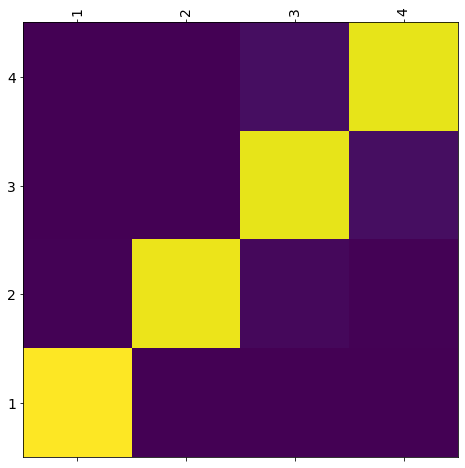
BONUS 1: DEPICT THE ATTENTION

For a sample input, we will record the attention values for each time step
Then, we will use the color codes to depict the relation between inputs and outputs
The lighter colors indicate higher values (attention)
That is, the model pays more attention to some inputs when creating each output (prediction)
The model learns where to look for to create the output!

def evaluate(seq_in):
  attention_plot = np.zeros((n_timesteps_in, n_timesteps_in))
  print ('attention_plot shape: (n_timesteps_in, n_timesteps_in) {}'.format(attention_plot.shape))


  #sequence = [7, 9, 8, 5]
  sequence = one_hot_encode(seq_in,n_features)
  encoder_inputs=array(sequence).reshape(1,n_timesteps_in,n_features)
  
  encoder_inputs = tf.convert_to_tensor(encoder_inputs,dtype=tf.float32)
  print ('Encoder input shape: (batch size, sequence length, n_features) {}'.format(encoder_inputs.shape))


  encoder_outputs, state_h, state_c = encoder_lstm(encoder_inputs)

  print ('Encoder output shape: (batch size, sequence length, latentSpaceDimension) {}'.format(encoder_outputs.shape))
  print ('Encoder Hidden state shape: (batch size, latentSpaceDimension) {}'.format(state_h.shape))
  print ('Encoder Cell state shape: (batch size, latentSpaceDimension) {}'.format(state_c.shape))
  # initial context vector is the states of the encoder
  states = [state_h, state_c]
  
  # Set up the attention layer
  #attention= BahdanauAttention(latentSpaceDimension)


  # Set up the decoder layers
  #decoder_inputs = Input(shape=(1, (n_features+latentSpaceDimension)))
  #decoder_lstm = LSTM(latentSpaceDimension,  return_state=True, name='decoder_lstm')
  #decoder_dense = Dense(n_features, activation='softmax',  name='decoder_dense')

  all_outputs = []

  #INIT DECODER
  # Prepare decoder input data that just contains the start character 0
  # Note that we made it a constant one-hot-encoded in the model
  # that is, [1 0 0 0 0 0 0 0 0 0] is the first input for each loop
  decoder_input_data = np.zeros((1, 1, n_features))
  decoder_input_data[:, 0, 0] = 1 
  # that is, [1 0 0 0 0 0 0 0 0 0] is the first input for each loop
  inputs = decoder_input_data
  #initial hiiden state
  decoder_outputs = state_h

  print('initial decoder inputs: ', inputs.shape)

  # decoder will only process one timestep at a time.
  for t in range(n_timesteps_in):

      # pay attention
      context_vector, attention_weights=attention(decoder_outputs, encoder_outputs)



      print("Attention context_vector: (batch size, units) {}".format(context_vector.shape))
      print("Attention weights : (batch_size, sequence_length, 1) {}".format(attention_weights.shape))

      # storing the attention weights to plot later on
      attention_weights = tf.reshape(attention_weights, (-1, ))
      attention_plot[t] = attention_weights.numpy()

      
      decoder_outputs=tf.expand_dims(decoder_outputs, 1)
      print('decoder_outputs: (batch_size, 1, latentSpaceDimension) ', decoder_outputs.shape )

      context_vector = tf.expand_dims(context_vector, 1)
      print('Reshaped context_vector: ', context_vector.shape )
      inputs = tf.concat([context_vector, inputs], axis=-1)
      #inputs = tf.concat([context_vector, inputs], axis=-1)
      print('After concat inputs: (batch_size, 1, n_features + hidden_size): ',inputs.shape )

      # passing the concatenated vector to the LSTM
      # Run the decoder on one timestep
      decoder_outputs, state_h, state_c = decoder_lstm(inputs,
                                              initial_state=states)
      #decoder_outputs = tf.reshape(decoder_outputs, (-1, decoder_outputs.shape[2]))
    
      outputs = decoder_dense(decoder_outputs)
      # Store the current prediction (we will concatenate all predictions later)
      outputs = tf.expand_dims(outputs, 1)
      all_outputs.append(outputs)
      # Reinject the outputs as inputs for the next loop iteration
      # as well as update the states
      inputs = outputs
      states = [state_h, state_c]



  # Concatenate all predictions such as [batch_size, timesteps, features]
  decoder_outputs = Lambda(lambda x: K.concatenate(x, axis=1))(all_outputs)
  seq_out=one_hot_decode(decoder_outputs[0])
  
  return seq_in, seq_out, attention_plottime: 63.8 ms# function for plotting the attention weights
def plot_attention(attention, sequence, predicted_sequence):
  fig = plt.figure(figsize=(8,8))
  ax = fig.add_subplot(1, 1, 1)
  ax.matshow(attention, cmap='viridis')

  fontdict = {'fontsize': 14}

  ax.set_xticklabels([''] + sequence, fontdict=fontdict, rotation=90)
  ax.set_yticklabels([''] + predicted_sequence, fontdict=fontdict)

  ax.xaxis.set_major_locator(ticker.MultipleLocator(1))
  ax.yaxis.set_major_locator(ticker.MultipleLocator(1))

  plt.show()time: 10.3 msdef translate(seq_in):
  seq_in, seq_out, attention_plot = evaluate(seq_in)

  print('Input: %s' % (seq_in))
  print('Predicted translation: {}'.format(seq_out))

  attention_plot = attention_plot[:len(seq_out), :len(seq_in)]
  plot_attention(attention_plot, seq_in, seq_out)time: 3.59 ms#translate([1, 2, 3 ,4,5,6,7,8,9,1,2,3,4,5,7,6])
translate([1, 2, 3 ,4])Input: [1, 2, 3, 4]
Predicted translation: [4, 3, 2, 1]

time: 176 ms

BONUS 2: LUONG ATTENTION

As we discussed, the only difference between Bahdanau and Luong Attention is the calculation of the score.

Here we use the dot product for finding the score as suggested by Luong et.al.

#LUONGH Dot-product score = tf.transpose(tf.matmul(query_with_time_axis, values_transposed) , perm=[0, 2, 1])

class LuongAttention(tf.keras.layers.Layer):
  def __init__(self, units):
    super(LuongAttention, self).__init__()
    self.W1 = tf.keras.layers.Dense(units)
    self.W2 = tf.keras.layers.Dense(units)
    self.V = tf.keras.layers.Dense(1)

  def call(self, query, values):
    print('\n******* Luong Attention  STARTS******')
    print('query (decoder hidden state): (batch_size, hidden size) ', query.shape)
    print('values (encoder all hidden state): (batch_size, max_len, hidden size) ', values.shape)

    # query hidden state shape == (batch_size, hidden size)
    # query_with_time_axis shape == (batch_size, 1, hidden size)
    # values shape == (batch_size, max_len, hidden size)
    # we are doing this to broadcast addition along the time axis to calculate the score
    query_with_time_axis = tf.expand_dims(query, 1)
    
    print('query_with_time_axis:(batch_size, 1, hidden size) ', query_with_time_axis.shape)


    values_transposed = tf.transpose(values, perm=[0, 2, 1])
    print('values_transposed:(batch_size, hidden size, max_len) ', values_transposed.shape)

    # score shape == (batch_size, max_length, 1)
    # we get 1 at the last axis because we are applying score to self.V
    # the shape of the tensor before applying self.V is (batch_size, max_length, units)
    #BAHDANAU ADDITIVE:
    #score = self.V(tf.nn.tanh(
    #    self.W1(query_with_time_axis) + self.W2(values)))
    
    #LUONGH Dot-product
    score = tf.transpose(tf.matmul(query_with_time_axis, values_transposed) , perm=[0, 2, 1])

    print('score: (batch_size, max_length, 1) ',score.shape)
    # attention_weights shape == (batch_size, max_length, 1)
    attention_weights = tf.nn.softmax(score, axis=1)
    print('attention_weights: (batch_size, max_length, 1) ',attention_weights.shape)
    # context_vector shape after sum == (batch_size, hidden_size)
    context_vector = attention_weights * values
    print('context_vector before reduce_sum: (batch_size, max_length, hidden_size) ',context_vector.shape)
    context_vector = tf.reduce_sum(context_vector, axis=1)
    print('context_vector after reduce_sum: (batch_size, hidden_size) ',context_vector.shape)


    print('\n******* Luong Attention ENDS******')
    return context_vector, attention_weights

WRAP UP

We have discussed Encoder-Decoder Model and observed that when the input sequence gets longer Encoder-Decoder model can not relate the output to the input successfully
We have seen that we can relate each output with each input by using an attention mechanism.
In the experiments, the positive effect of the attention mechanism on performance is clear.
We implemented Bahdanau style (Additive) attention which is a global attention mechanism.
Another global attention mechanism is Luong Attention (Multiplicative) in which only the calculation of the score values differs.
If only the dot product was used in Luong Attention (Multiplicative), it would be more efficient in terms of score calculations
We can summarize the methods to find score values below: